Data Scource and Exploratory Data Analysis
Shiyuan Zhou
Data Source
The Data that I used to answer my research question is based on the WHO data and published on Kaggle by Kumar Rajarshi. This dataset includes values social factors of 193 countries from 2000 to 2015 and the life expectancy in age. In our research question, we are aim to compare the impact of government health expenditure and Human Development Index on life expectancy. These two predictors are represent by ‘Total expenditure’ and ‘Income composition of resources’ in our data-set. The target is life expectancy. Since we also stated that social factors may have a big difference between developed and developing countries. We sill also include the binary variable ‘Status’ that indicate the development status of a country. All of these variables will change across years.
Link of data: https://www.kaggle.com/kumarajarshi/life-expectancy-who
We also used a data-set that help us in visualizations from: https://www.kaggle.com/datasets/andradaolteanu/country-mapping-iso-continent-region?resource=download. This is not our main data and all the data exploration part is focusing on our previous main data.
Exploratory Data Analysis
Before answering our research question, we need to do Exploratory Data Analysis first to find issues in our data, clean our data, and make summary statistics, plots, and graphs for our key variables.
Data Checking
| num_na | |
|---|---|
| Country | 0 |
| Year | 0 |
| Status | 0 |
| Life expectancy | 10 |
| Adult Mortality | 10 |
| infant deaths | 0 |
| Alcohol | 193 |
| percentage expenditure | 0 |
| Hepatitis B | 553 |
| Measles | 0 |
| BMI | 34 |
| under-five deaths | 0 |
| Polio | 19 |
| Total expenditure | 225 |
| Diphtheria | 19 |
| HIV/AIDS | 0 |
| GDP | 448 |
| Population | 652 |
| thinness 1-19 years | 34 |
| thinness 5-9 years | 34 |
| Income composition of resources | 167 |
| Schooling | 163 |
We have 2937 number of observations and 22 number of variables in our dataset. There are 14 columns contain NAs. There are 167 missing values in Income composition of resources and 225 NAs in total expenditure. The variable with highest amount of NAs is ‘Hepatitis B’. We will do the missing value imputation in the next section.
Check dimensions of our data
| axis | value |
|---|---|
| num_observations | 2937 |
| num_variables | 22 |
We have 2937 number of observations and 22 number of variables in our dataset.
Check the summary statistics of required numeric variables
| Life expectancy | Adult Mortality | Total expenditure | HIV/AIDS | Income composition of resources | |
|---|---|---|---|---|---|
| Min. :36.30 | Min. : 1.0 | Min. : 0.370 | Min. : 0.100 | Min. :0.0000 | |
| 1st Qu.:63.10 | 1st Qu.: 74.0 | 1st Qu.: 4.260 | 1st Qu.: 0.100 | 1st Qu.:0.4930 | |
| Median :72.10 | Median :144.0 | Median : 5.755 | Median : 0.100 | Median :0.6770 | |
| Mean :69.22 | Mean :164.8 | Mean : 5.938 | Mean : 1.743 | Mean :0.6275 | |
| 3rd Qu.:75.70 | 3rd Qu.:228.0 | 3rd Qu.: 7.492 | 3rd Qu.: 0.800 | 3rd Qu.:0.7790 | |
| Max. :89.00 | Max. :723.0 | Max. :17.600 | Max. :50.600 | Max. :0.9480 | |
| NA’s :10 | NA’s :10 | NA’s :225 | NA | NA’s :167 |
Since our data-set contains multiple variables, presenting summary statistics for all the variables is not optimal. Here are the summary statistics of several key variables help us to find the issues and reliability of our data. According to the summary table we get, variable ‘Life expectancy’ and ‘Total expenditure’ do not have big issues and in our estimated bound(life expectancy should be greater than 0 and less than 100, total expenditure should be greater than 0 and less than 100 since it represents proportion). However, the variable ‘income composition of resources’ has minimum values equals to 0. Since this variable indicate human development index, its impossible to have 0 values, which means we need to remove those observations. According to the worldpopulationreview.com, the country with lowest HDI in 2019 is Niger with 0.394. Hence, 0 income composition should be removed from the data set in order to prevent wrong model fitting. Other variables’ reliability were also checked.
Check Distribution of required variables
The distribution of several main variables are checked base on their plotted histograms.
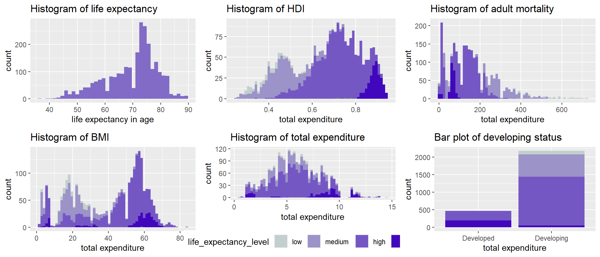 To have more insights on their relationship with life expectancy, we also made variable ‘life_expectancy_level’ for different levels of ages only for EDA. The distribution of life expectancy and total expenditure is quite normal but life expectancy is left-skewed. For HDI(Income composition of resources) and BMI, we can see that, higher level of life expectancy concentrated on higher HDI, which may indicate a positive relationship. For adult mortality records, low mortality may have higher life expectancy as the distribution of color goes darker from right to left. FUrthermore, developed country tend to have higher life expectancy. There were no too much clear relationship in other variables.
Data Wrangling
NA Imputation and data joining
We handled the missing values by imputation. We use mean value of current column to impute by for looping each column. In the visualization part, we also used countries’ sub region of their continent. Hence, we made a left join on our main data-set with continent data-set by each country’s name.
Create New Variable
We handled the missing values by imputation. We use mean value of current column to impute by for looping each column.
To do further data exploration on different types of plots, we need both numeric and categorical ‘Total expenditure’ and ‘Income composition of resources’. Converting current numeric variables to categorical variables helps us on stacked histograms, statistical summary graph, and etc. In many statistical research on social factors, health expenditure and HDI are always represented by different levels.
Create a new categorical variable named “expenditure_level” using total expenditure on health of a country. (rare total expenditure < 3; low total expenditure 3-5; mild total expenditure 5-9; high total expenditure > 9) and a new categorical variable named “hdi_level” indicating level of income composition of resources of countries(low income composition < 0.55; medium income composition 0.55-0.7; high income composition 0.7-0.8; very high income composition > 0.8). Additionally, we should use factor() function to give our levels an order for future convenience.
Since we also need to perform gradient boosting and extreme gradient boosting to predict life expectancy based on our dataset. Hence, we need to make character variables into numeric variables since boosting model cannot apply to categorical variables. By looking at the dataset, we found that variable ‘Status’ and ‘Country’ are categorical. We do not need variable ‘Country’ in machine learning model fitting as we investigate the dataset as a whole: each country’s value in each year is a single observation. Variable ‘Status’ is binary. Hence, we only need to convert it into 1 and 0 and create new variables ‘status_num’.
We also found the range of variable ‘GDP’, ‘Percentage Expenditure’ and ‘Population’ are much larger than other variables, which means we need to scale them. If there is a big difference in the range of variables, higher ranging numbers may have superiority in model fitting.
| expenditure_level | min_exp | max_exp | count |
|---|---|---|---|
| low | 0.37 | 2.98 | 276 |
| medium | 3.00 | 5.00 | 652 |
| high | 5.10 | 8.99 | 1464 |
| very high | 9.10 | 14.39 | 248 |
| hdi_level | min_exp | max_exp | count |
|---|---|---|---|
| low | 0.253 | 0.548 | 720 |
| medium | 0.550 | 0.700 | 703 |
| high | 0.701 | 0.800 | 668 |
| very high | 0.801 | 0.948 | 549 |
Copyright © 2022, Shiyuan(Eric) Zhou.